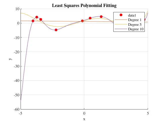
Understanding Least Squares Polynomial Fitting
When you have a bunch of points on a plot and you need to find a smooth curve that best fits those points, you’re dealing with a classic problem in mathematics and engineering. This is where polynomial fitting using the least squares method comes into play. Imagine these points as the marks on your dartboard. You’re trying to find the best path that goes near most of these marks.
The Heart of the Matter: Least Squares
Picture this: Once you’ve chosen a polynomial (say, a curve), for each of your data points (), there’s a difference (or “residual”) between the actual value and the value predicted by your curve. If we take all these differences for all points and square them (because we don’t want negative distances messing things up), and then add these squares together, we get a single giant number that tells us how “off” our curve is. This is our sum of squares.
Optimizing the Fit
Our mission is to make this sum of squares as small as possible. Why? Because the smaller this sum, the closer our curve is to those data points - it’s as simple as that. This optimization problem might sound daunting, but it turns into a manageable set of equations once we express our polynomial in an algebraic form, associating it with matrices. Our polynomial’s coefficients become variables in these equations.
Behind the Scenes
To solve this optimization problem and find these coefficients that give us the minimum sum of squares, we use a bit of matrix algebra magic—one method involves the “normal equation” , where is a matrix containing powers of values, is our sought-after coefficient vector, and is our vector of observed values.
Why does this approach work? Because when you set up and solve these equations, they inherently find the point where our sum of squares is at its lowest—the optimal fit for our data.
Why This Method Works
The least squares method doesn’t just chase after one point, trying to minimize the distance from it; instead, it considers all the poaints simultaneously, ensuring the final curve respects the overall trend of the data rather than getting overly distracted by outliers. This way, we get a polynomial that smoothly follows the general direction of our data points.
By embracing a combination of calculus and linear algebra, we turn a seemingly complex problem into something neatly solvable, providing a robust tool for data analysis and modeling in countless applications.

In essence, the least squares method provides us with a systematic way to strike a balance between fitting as close as possible to all points while smoothing out the noise. It’s this equilibrium between fidelity to the data and simplicity of the model that makes the least squares method so widely applicable and powerful.