ENSC 380 MATLAB Assignment 1

Kavahn Ahluwalia 3015810333

2: Continuous-time signals

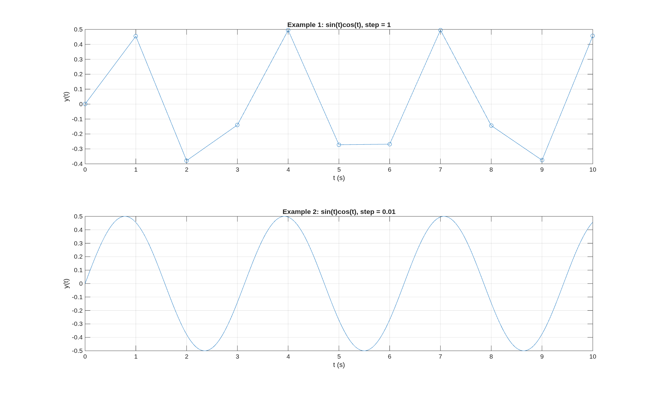
MATLAB can’t store a real continuous time function, so we plot connects them with straight lines. With a step of 1 (Example 1) you can see the straight segments. With a step of 0.01 (Example 2) it looks continuous.

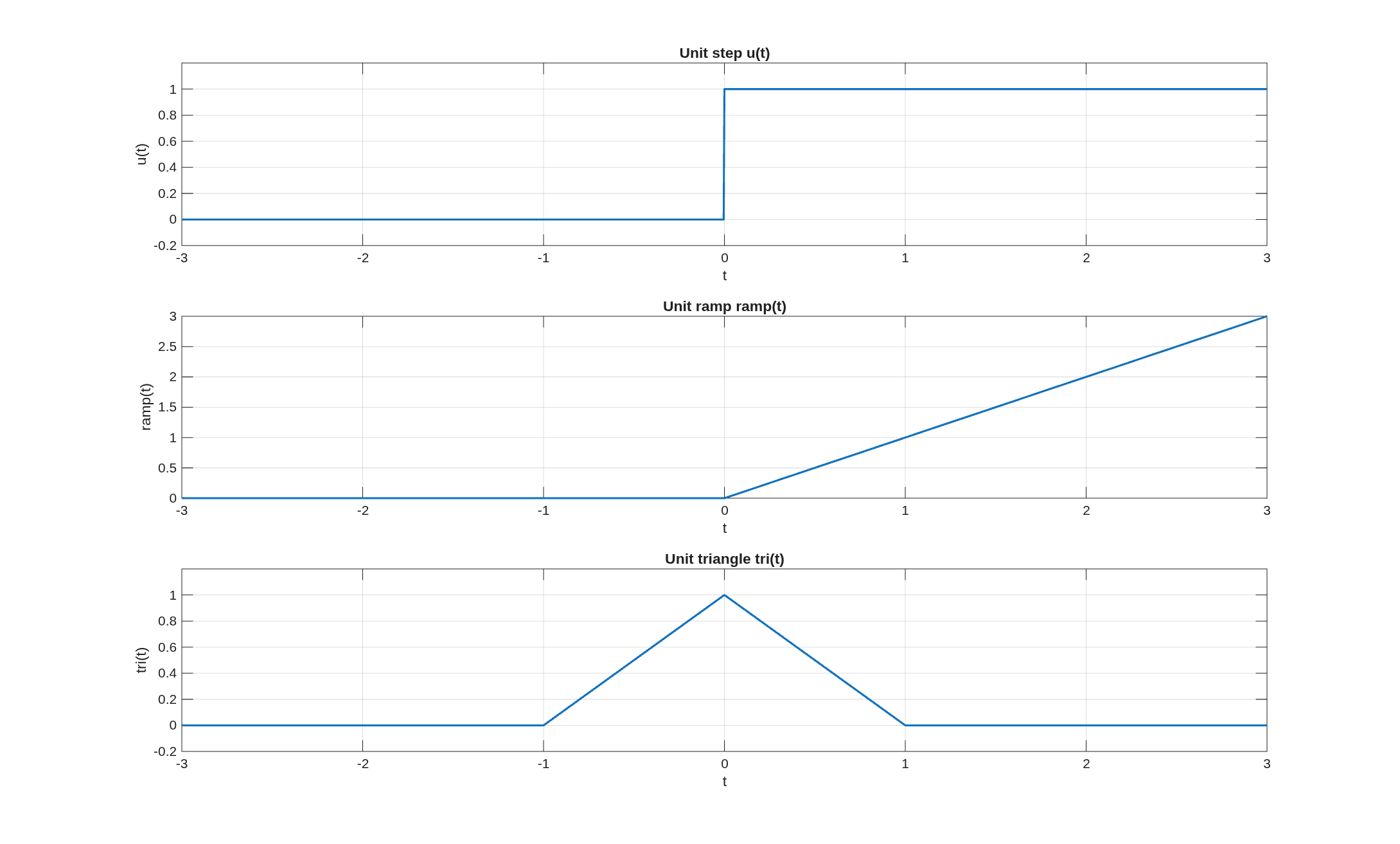
Unit step, ramp and triangle

These aren’t built into MATLAB, so we wrote them as function files:

u (t) = {1, 0, t \geq 0 t < 0 ramp (t) = t u (t) tri (t) = {1 - ∣ t ∣, 0, ∣ t ∣ < 1 otherwise

u.m

 
function y = u(t)
 
% unit step
 
y = double(t >= 0);
 
end

ramp.m

 
function y = ramp(t)
 
% unit ramp
 
y = t .* u(t);
 
end

tri.m

 
function y = tri(t)
 
% unit triangle
 
y = (1 - abs(t)) .* (abs(t) < 1);
 
end

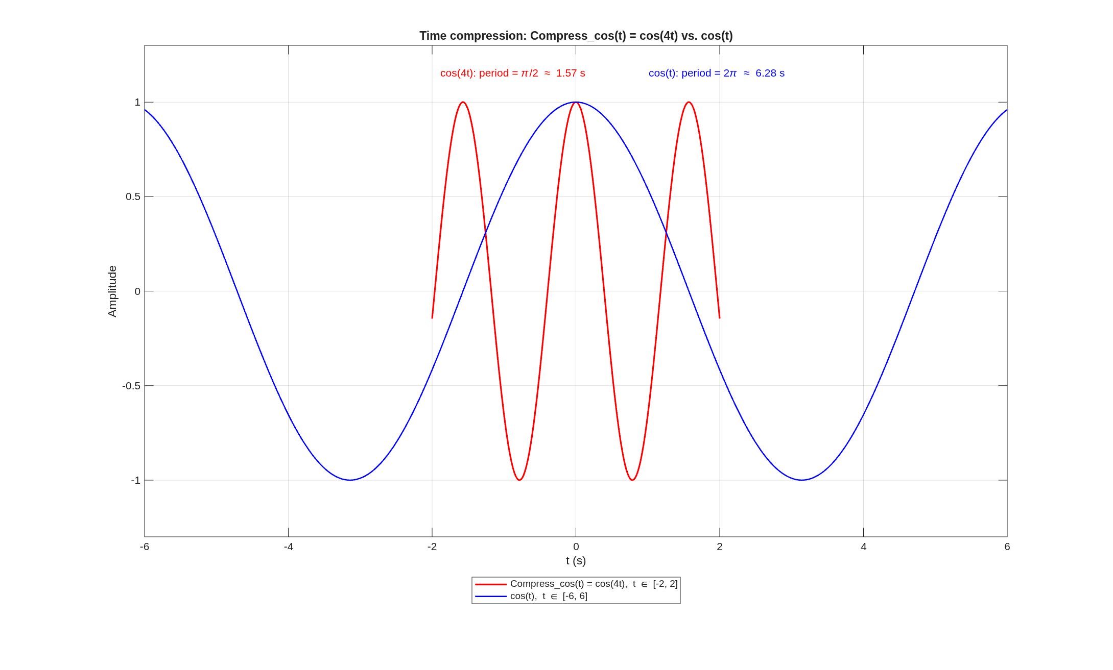
Compress_cos(t) = cos(4t)

Compress_cos.m

 
function y = Compress_cos(t)
 
y = cos(4*t);
 
end

Replacing $t$ with $4 t$ compresses the signal in time by 4, so the period goes from $2 π \approx 6.28$ s to

$T = \frac{2 π}{4} = \frac{π}{2} \approx 1.57 s$

On $[- 2, 2]$ the red curve gets through about 2.5 periods, while the blue $cos (t)$ does less than 2 periods over all of $[- 6, 6]$ . The amplitude stays the same.

Full code for step 2:
part2_continuous.m

 
%% ENSC 380 - MATLAB Assignment 1, Step 2
 
clear; clc; close all;
 
  
 
% examples 1 and 2
 
t1 = 0:1:10;
 
y1 = sin(t1).*cos(t1);
 
t2 = 0:0.01:10;
 
y2 = sin(t2).*cos(t2);
 
  
 
figure(Theme="light");
 
subplot(2,1,1);
 
plot(t1, y1, 'o-'); grid on;
 
title('Example 1: sin(t)cos(t), step = 1');
 
xlabel('t (s)'); ylabel('y(t)');
 
subplot(2,1,2);
 
plot(t2, y2); grid on;
 
title('Example 2: sin(t)cos(t), step = 0.01');
 
xlabel('t (s)'); ylabel('y(t)');
 
saveas(gcf, 'figures/step2_examples.png');
 
  
 
% testing u, ramp and tri
 
t = -3:0.001:3;
 
figure(Theme="light");
 
subplot(3,1,1);
 
plot(t, u(t)); grid on; ylim([-0.2 1.2]);
 
title('Unit step u(t)'); xlabel('t'); ylabel('u(t)');
 
subplot(3,1,2);
 
plot(t, ramp(t)); grid on;
 
title('Unit ramp ramp(t)'); xlabel('t'); ylabel('ramp(t)');
 
subplot(3,1,3);
 
plot(t, tri(t)); grid on; ylim([-0.2 1.2]);
 
title('Unit triangle tri(t)'); xlabel('t'); ylabel('tri(t)');
 
saveas(gcf, 'figures/step2_u_ramp_tri.png');
 
  
 
% Compress_cos vs cos
 
t1 = -2:0.001:2;
 
t2 = -6:0.001:6;
 
figure(Theme="light");
 
plot(t1, Compress_cos(t1), 'r');
 
hold on;
 
plot(t2, cos(t2), 'b');
 
hold off; grid on;
 
ylim([-1.3 1.3]);
 
title('Step 2: Compress\_cos(t) = cos(4t) and cos(t)');
 
xlabel('t (s)'); ylabel('Amplitude');
 
legend('Compress\_cos(t) = cos(4t), -2 \leq t \leq 2', 'cos(t), -6 \leq t \leq 6', 'Location', 'southoutside');
 
text(-1.9, 1.15, 'period = \pi/2', 'Color', 'r');
 
text(2.5, 1.15, 'period = 2\pi', 'Color', 'b');
 
saveas(gcf, 'figures/step2_compress_cos.png');

3: Discrete time signals

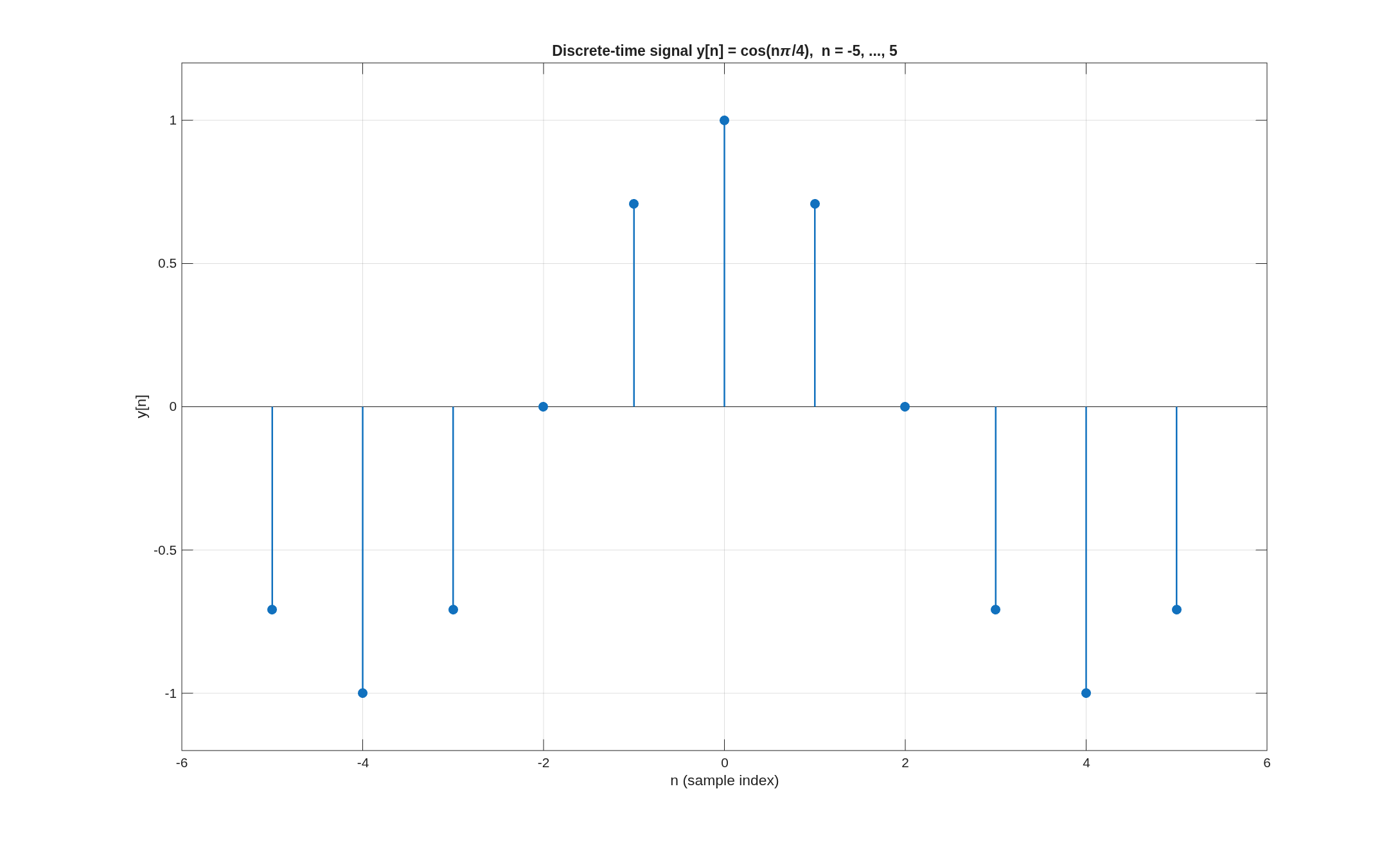
$y [n] = cos (nπ /4)$ only exists at the integers $n = - 5, \dots, 5$ , so we used stem. The axis goes from $- 6$ to $6$ just so the plot isn’t cut off at the edges.

The period is $N = \frac{2 π}{π /4} = 8$ samples, which is why $y [0] = 1$ and $y [\pm 4] = - 1$ .
part3_discrete.m

 
%% ENSC 380 - MATLAB Assignment 1, Step 3
 
clear; clc; close all;
 
  
 
n = -5:5;
 
y = cos(n*pi/4);
 
  
 
figure(Theme="light");
 
stem(n, y, 'filled'); grid on;
 
xlim([-6 6]); ylim([-1.2 1.2]);
 
title('Step 3: y[n] = cos(n\pi/4)');
 
xlabel('n'); ylabel('y[n]');
 
saveas(gcf, 'figures/step3_discrete_cos.png');

4: Wave file

I used the clip given with the assignment (tara.wav), saved as original-clip.wav. It’s 8 kHz, 8-bit, mono, 7.13 s and 57 kB, which fits the 4–10 s and 30–100 kB range.

Step 5: Reading the file

 
[y, fs] = audioread('original-clip.wav');
 
info = audioinfo('original-clip.wav');

What does fs do? fs is the sampling frequency, the number of samples per second taken when the sound was recorded. Samples in y are $1/ f_{s}$ seconds apart.

Value of fs: 8000 Hz, so the samples are 125 µs apart.

audioinfo: Duration = 7.1315 s, BitsPerSample = 8.

6: Playing the file

 
sound(y, fs);

It sounds the same as the original, since it’s played back at the same 8 kHz rate it was recorded at.

7: Plotting the audio

 
plot((1:1:length(y))/fs, y);

Dividing the sample number by $f_{s}$ puts the x-axis in seconds.

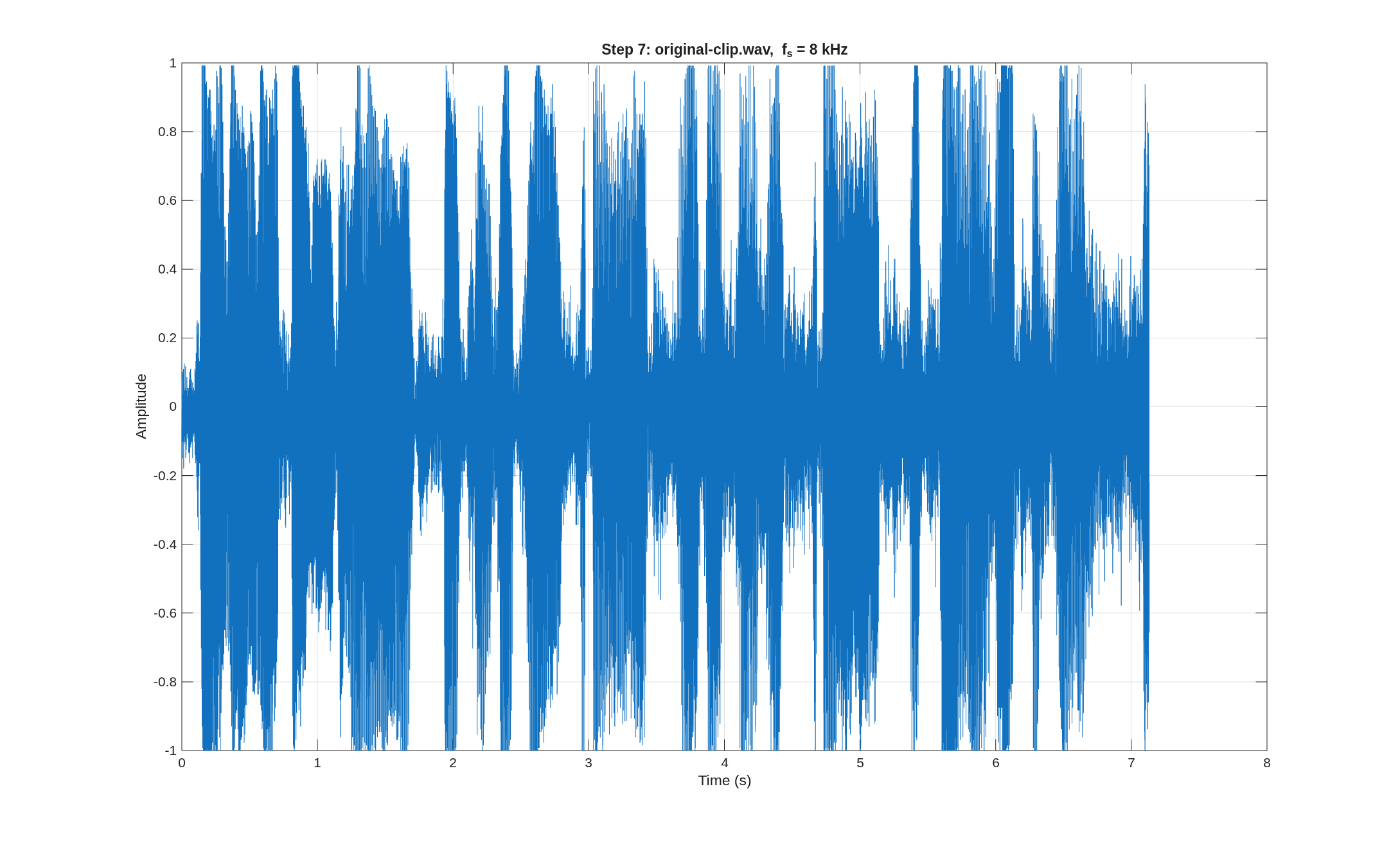
Length of the clip: $57052/8000 = 7.13$ s, the same as audioinfo gave.

8: Changing the volume

 
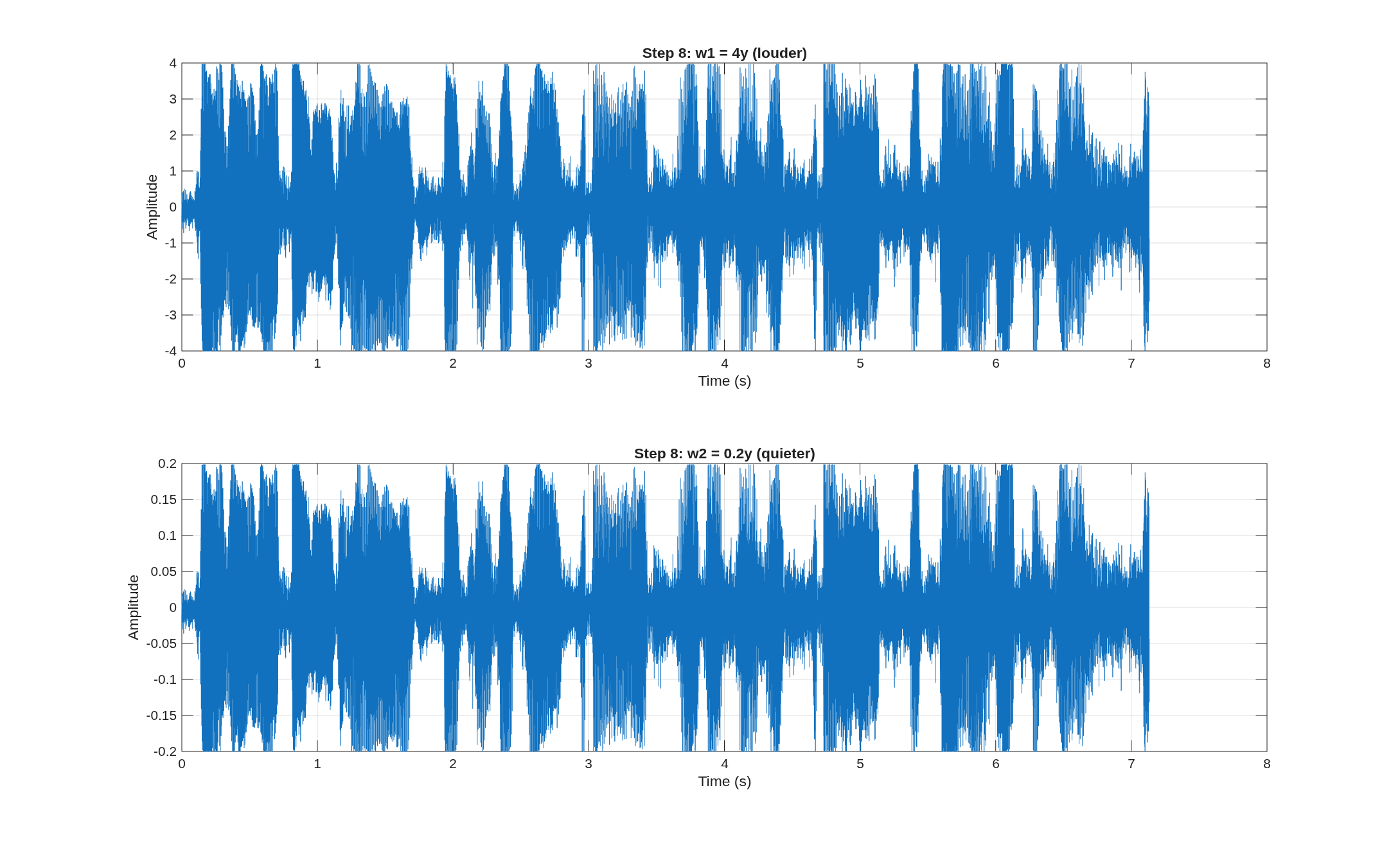
w1 = 4*y;
 
w2 = 0.2*y;

w1 is louder (4x the amplitude, about +12 dB). Since y already goes up to ±1, a lot of w1 goes past $[- 1, 1]$ and clips when it plays, so it sounds distorted. w2 is quieter (about −14 dB) but otherwise sounds the same.

9: Stretching and compressing

We don’t have the Signal Processing Toolbox, so instead of upsample and downsample we did it with indexing:

 
w3 = zeros(2*length(y), 1);
 
w3(1:2:end) = y;
 
w4 = y(1:3:end);
 
audiowrite('w3.wav', w3, fs);
 
audiowrite('w4.wav', w4, fs);

The handout has audiowrite(w3,fs,'w3.wav'), but that gives an error. The right order is audiowrite(filename, y, fs).

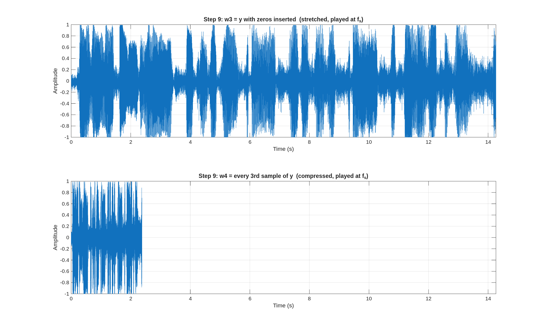
Lengths at 8000 Hz: w3 is $114104/8000 = 14.26$ s (twice the original) and w4 is $19018/8000 = 2.38$ s (a third of the original).

How they sound: w3 plays at half speed and the voice is deeper, because every frequency is halved. Putting in zeros instead of interpolating also leaves a mirrored copy of the spectrum in the 2–4 kHz range, so there’s a high pitched sound on top of the voice.

w4 plays 3 times faster and sounds like a chipmunk, because every frequency is tripled. We didn’t filter before dropping samples, so anything above $\frac{8000}{2 \cdot 3} \approx 1.33$ kHz aliases back down, which makes it distorted and harder to understand.

This is time scaling $x (a t)$ : w3 played at $f_{s}$ is $y (t /2)$ ( $a = \frac{1}{2}$ , expansion) and w4 is $y (3 t)$ ( $a = 3$ , compression).

Full code for steps 5 to 9:

part5to9_audio.m

 
%% ENSC 380 - MATLAB Assignment 1, Steps 5 to 9
 
clear; clc; close all;
 
  
 
%% Step 5
 
[y, fs] = audioread('original-clip.wav');
 
fs
 
info = audioinfo('original-clip.wav');
 
info.Duration
 
info.BitsPerSample
 
  
 
%% Step 6
 
sound(y, fs);
 
pause(length(y)/fs + 1);
 
  
 
%% Step 7
 
t = (1:1:length(y))/fs;
 
figure(Theme="light");
 
plot(t, y); grid on;
 
title('Step 7: original-clip.wav');
 
xlabel('Time (s)'); ylabel('Amplitude');
 
saveas(gcf, 'figures/step7_original.png');
 
  
 
clip_length = length(y)/fs
 
  
 
%% Step 8
 
w1 = 4*y;
 
w2 = 0.2*y;
 
  
 
figure(Theme="light");
 
subplot(2,1,1);
 
plot(t, w1); grid on;
 
title('Step 8: w1 = 4y'); xlabel('Time (s)'); ylabel('Amplitude');
 
subplot(2,1,2);
 
plot(t, w2); grid on;
 
title('Step 8: w2 = 0.2y'); xlabel('Time (s)'); ylabel('Amplitude');
 
saveas(gcf, 'figures/step8_volume.png');
 
  
 
sound(w1, fs);
 
pause(length(w1)/fs + 1);
 
sound(w2, fs);
 
pause(length(w2)/fs + 1);
 
  
 
%% Step 9
 
% don't have the signal processing toolbox so did upsample/downsample by hand
 
w3 = zeros(2*length(y), 1);
 
w3(1:2:end) = y;
 
w4 = y(1:3:end);
 
  
 
t3 = (1:length(w3))/fs;
 
t4 = (1:length(w4))/fs;
 
  
 
figure(Theme="light");
 
subplot(2,1,1);
 
plot(t3, w3); grid on; xlim([0 15]);
 
title('Step 9: w3 (stretched)'); xlabel('Time (s)'); ylabel('Amplitude');
 
subplot(2,1,2);
 
plot(t4, w4); grid on; xlim([0 15]);
 
title('Step 9: w4 (compressed)'); xlabel('Time (s)'); ylabel('Amplitude');
 
saveas(gcf, 'figures/step9_w3_w4.png');
 
  
 
w3_length = length(w3)/fs
 
w4_length = length(w4)/fs
 
  
 
sound(w3, fs);
 
pause(length(w3)/fs + 1);
 
sound(w4, fs);
 
pause(length(w4)/fs + 1);
 
  
 
audiowrite('w3.wav', w3, fs);
 
audiowrite('w4.wav', w4, fs);

10: Single echo

An echo is just a quieter, delayed copy of the sound added to the original:

$z [n] = y [n] + a y [n - D]$
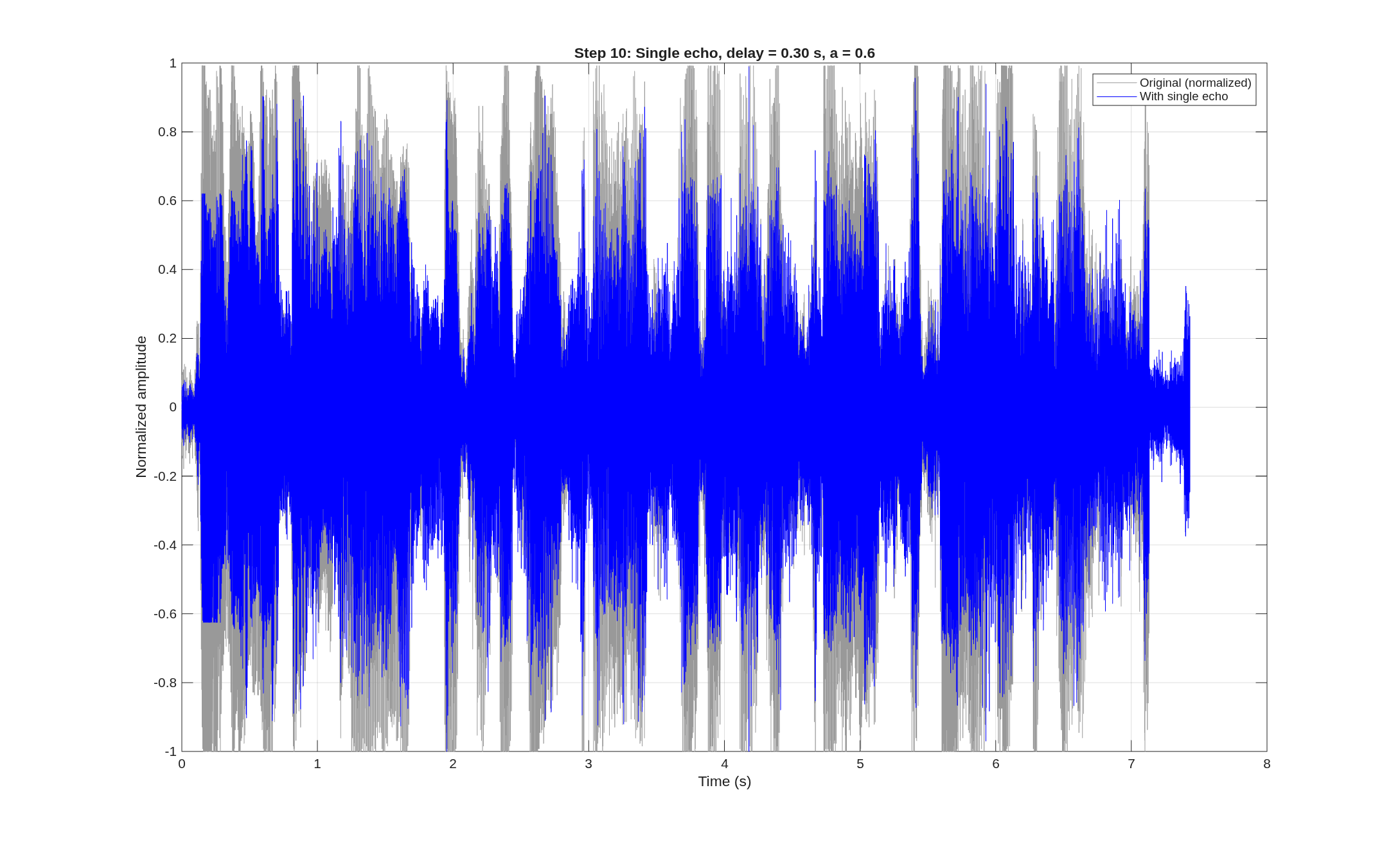
We used a 0.3 s delay ( $D = 0.3 \times 8000 = 2400$ samples) and $a = 0.6$ . The original gets $D$ zeros added at the end and the copy gets $D$ zeros at the start, so they’re the same length and the end of the echo isn’t cut off. Then we add them. The sum can go past $[- 1, 1]$ , so we normalize with z = z/max(abs(z)) before playing it and saving it with audiowrite.

It sounds like the clip was recorded in a big room, with every word repeated once, quieter, 0.3 s later. The impulse response is $h [n] = δ [n] + a δ [n - D]$ .

part10_echo_single.m

 
%% ENSC 380 - MATLAB Assignment 1, Step 10
 
clear; clc; close all;
 
  
 
[y, fs] = audioread('original-clip.wav');
 
  
 
delay = 0.3; % seconds
 
a = 0.6; % echo volume
 
D = round(delay*fs);
 
  
 
% pad both so they're the same length, then add the delayed copy
 
y1 = [y; zeros(D,1)];
 
y2 = [zeros(D,1); y];
 
z = y1 + a*y2;
 
  
 
z = z/max(abs(z)); % normalize so it doesn't clip
 
  
 
sound(z, fs);
 
audiowrite('echo_single.wav', z, fs);
 
  
 
t = (0:length(z)-1)/fs;
 
figure(Theme="light");
 
plot(t, z); grid on;
 
title('Step 10: Single echo (delay = 0.3 s, a = 0.6)');
 
xlabel('Time (s)'); ylabel('Amplitude');
 
saveas(gcf, 'figures/step10_echo_single.png');

11: Multiple echoes

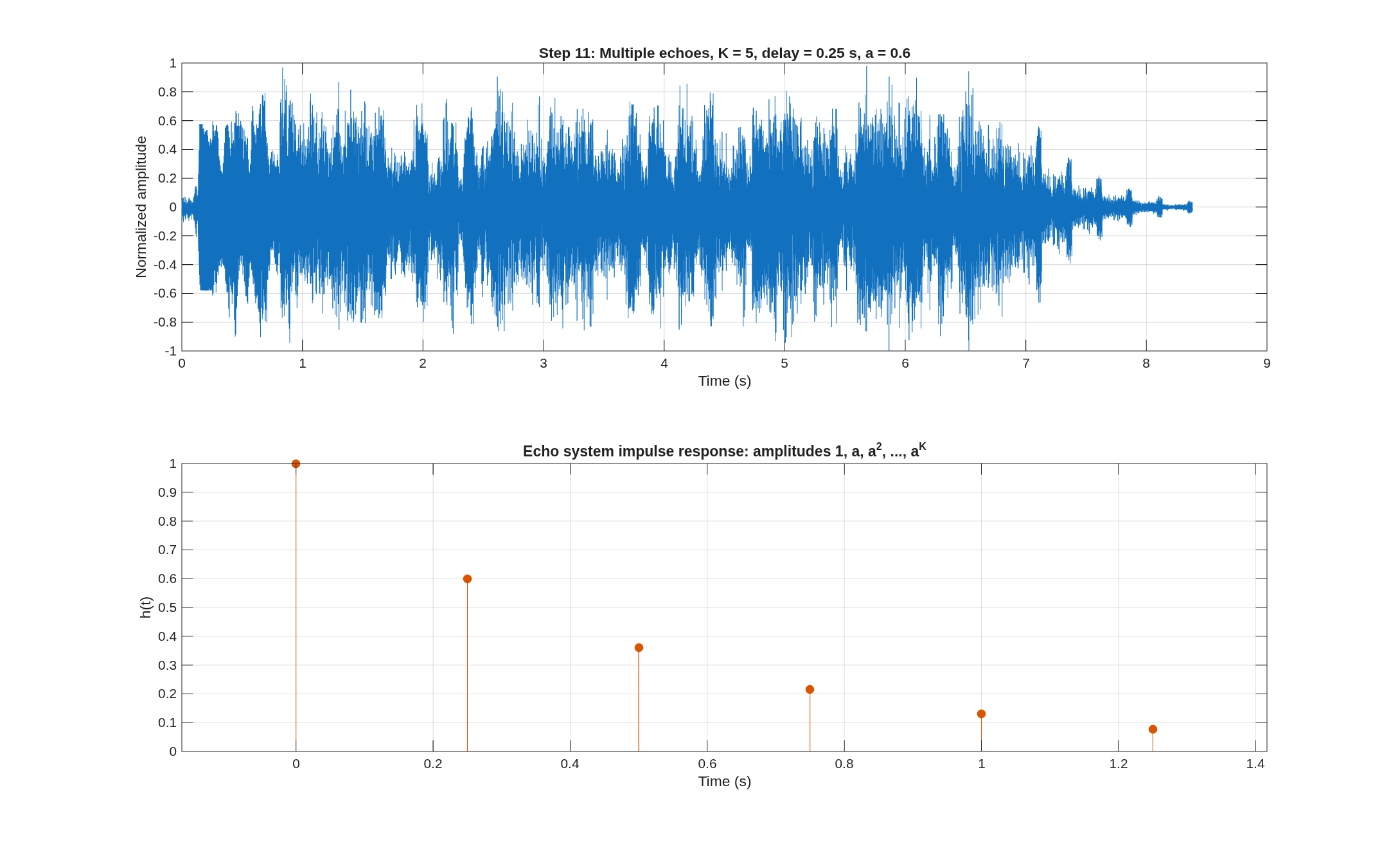
We added $K = 5$ echoes. Echo $k$ is delayed by $k D$ samples ( $D$ = 0.25 s = 2000 samples) and scaled by $a^{k}$ with $a = 0.6$ :
$z [n] = y [n] + \sum_{k = 1}^{5} a^{k} y [n - k D]$
So the echoes get quieter each time: $1, 0.6, 0.36, 0.216, 0.130, 0.078$ . We padded the output with $K D$ zeros so the last echo fits, added each echo in a for loop, and normalized at the end like in step 10.

Each word repeats a few times and fades out. The impulse response is $h [n] = \sum_{k = 0}^{5} a^{k} δ [n - k D]$ .

part11_echo_multiple.m

 
%% ENSC 380 - MATLAB Assignment 1, Step 11
 
clear; clc; close all;
 
  
 
[y, fs] = audioread('original-clip.wav');
 
  
 
delay = 0.25; % time between echoes (s)
 
a = 0.6;
 
K = 5; % number of echoes
 
D = round(delay*fs);
 
N = length(y);
 
  
 
z = [y; zeros(K*D,1)];
 
for k = 1:K
 
% each echo is delayed k*D samples and scaled by a^k
 
z(k*D+1 : k*D+N) = z(k*D+1 : k*D+N) + a^k*y;
 
end
 
  
 
z = z/max(abs(z));
 
  
 
sound(z, fs);
 
audiowrite('echo_multiple.wav', z, fs);
 
  
 
t = (0:length(z)-1)/fs;
 
figure(Theme="light");
 
plot(t, z); grid on;
 
title('Step 11: Multiple echoes (5 echoes, 0.25 s apart, a = 0.6)');
 
xlabel('Time (s)'); ylabel('Amplitude');
 
saveas(gcf, 'figures/step11_echo_multiple.png');

Kavahn's Notes

Explorer