ENSC 316 – Assignment 02 (MATLAB)
Q2 – Exercise 1.12: Charged hemisphere
Integral computed (ring at polar angle θ has radius a·sinθ, height a·cosθ, charge dQ = ρs·2πa²·sinθ dθ):
Evaluated with the midpoint rule over N rings.
% MATLAB Exercise 1.12 - Charged hemisphere, numerical integration in theta

%

% Ring at polar angle theta: radius a*sin(theta), height a*cos(theta),

% charge dQ = rho_s*2*pi*a^2*sin(theta)*dtheta. Summing the on-axis ring fields:

%

% Ez(z) = rho_s*a^2/(2*eps0) * Int_0^(pi/2) sin(theta)*(z - a*cos(theta))

% / (a^2 + z^2 - 2*a*z*cos(theta))^(3/2) dtheta

%

% evaluated with the midpoint rule (1.19) using N rings.

clear; clc;

eps0 = 8.8541878128e-12;


rhos = input('Surface charge density rho_s [C/m^2]: ');

a = input('Radius of the hemispherical shell a [m]: ');

z = input('z-coordinate of the field point [m]: ');

N = input('Number of rings N: ');


dtheta = (pi/2)/N;

theta = ((1:N) - 0.5)*dtheta; % centres of the N segments

f = sin(theta).*(z - a*cos(theta)) ./ (a^2 + z^2 - 2*a*z*cos(theta)).^1.5;

Enum = rhos*a^2/(2*eps0) * sum(f)*dtheta;


Ea = rhos*a^2/(2*eps0*z^2) * (a/sqrt(z^2 + a^2) + (z - a)/abs(z - a));

err = abs((Ea - Enum)/Ea)*100;


fprintf('\nNumerical Ez = %.6e V/m\n', Enum);

fprintf('Analytic Ez = %.6e V/m\n', Ea);

fprintf('Relative error = %.4e %%\n', err);
Output (ρs = 1e-9 C/m², a = 1 m, N = 500):
z = 5 m

Numerical Ez = 2.701811e+00 V/m

Analytic Ez = 2.701809e+00 V/m

Relative error = 6.5938e-05 %


z = 0.5 m

Numerical Ez = -2.384708e+01 V/m

Analytic Ez = -2.384698e+01 V/m

Relative error = 4.1740e-04 %
Q3 – Exercise 1.13: Line charge with quiver
% MATLAB Exercise 1.13 - E-field of a finite line charge (along x, centred

% at the origin) by numerical superposition of point charges, shown with quiver.

clear; clc;

eps0 = 8.8541878128e-12;

k = 1/(4*pi*eps0);


N = input('Number of subdivisions of the line N: ');

L = input('Length of the line L [cm]: ')/100;

Q = input('Total charge Q [nC]: ')*1e-9;


% 10 x 10 field-point grid; an even point count keeps y = 0 off the grid

[X, Y] = meshgrid(linspace(-0.6*L, 0.6*L, 10), linspace(-0.2*L, 0.2*L, 10));


dQ = Q/N;

xs = -L/2 + ((1:N) - 0.5)*L/N; % source points = segment centres

Ex = zeros(size(X));

Ey = zeros(size(X));

for i = 1:size(X, 1) % field point row

for j = 1:size(X, 2) % field point column

for n = 1:N % source point

Rx = X(i,j) - xs(n);

Ry = Y(i,j);

R3 = (Rx^2 + Ry^2)^1.5;

Ex(i,j) = Ex(i,j) + k*dQ*Rx/R3;

Ey(i,j) = Ey(i,j) + k*dQ*Ry/R3;

end

end

end


% Diagnostics: compare with the closed-form field of a finite line

lam = Q/L;

r1 = sqrt((X + L/2).^2 + Y.^2); % distance to left end

r2 = sqrt((X - L/2).^2 + Y.^2); % distance to right end

ExA = k*lam*(1./r2 - 1./r1);

EyA = k*lam./Y.*((X + L/2)./r1 - (X - L/2)./r2);

relErr = hypot(Ex - ExA, Ey - EyA)./hypot(ExA, EyA)*100;

fprintf('\nN = %d, L = %g m, Q = %g C\n', N, L, Q);

fprintf('|E| range on grid: %.4e to %.4e V/m\n', min(hypot(Ex,Ey),[],'all'), max(hypot(Ex,Ey),[],'all'));

fprintf('Max relative error vs analytic: %.4e %%\n', max(relErr, [], 'all'));


figure;

quiver(X, Y, Ex, Ey);

hold on;

plot([-L/2 L/2], [0 0], 'r', 'LineWidth', 3);

axis equal;

xlabel('x [m]'); ylabel('y [m]');

title(sprintf('E-field of a line charge (N = %d, Q = %g nC, L = %g cm)', N, Q*1e9, L*100));

legend('E', 'line charge');
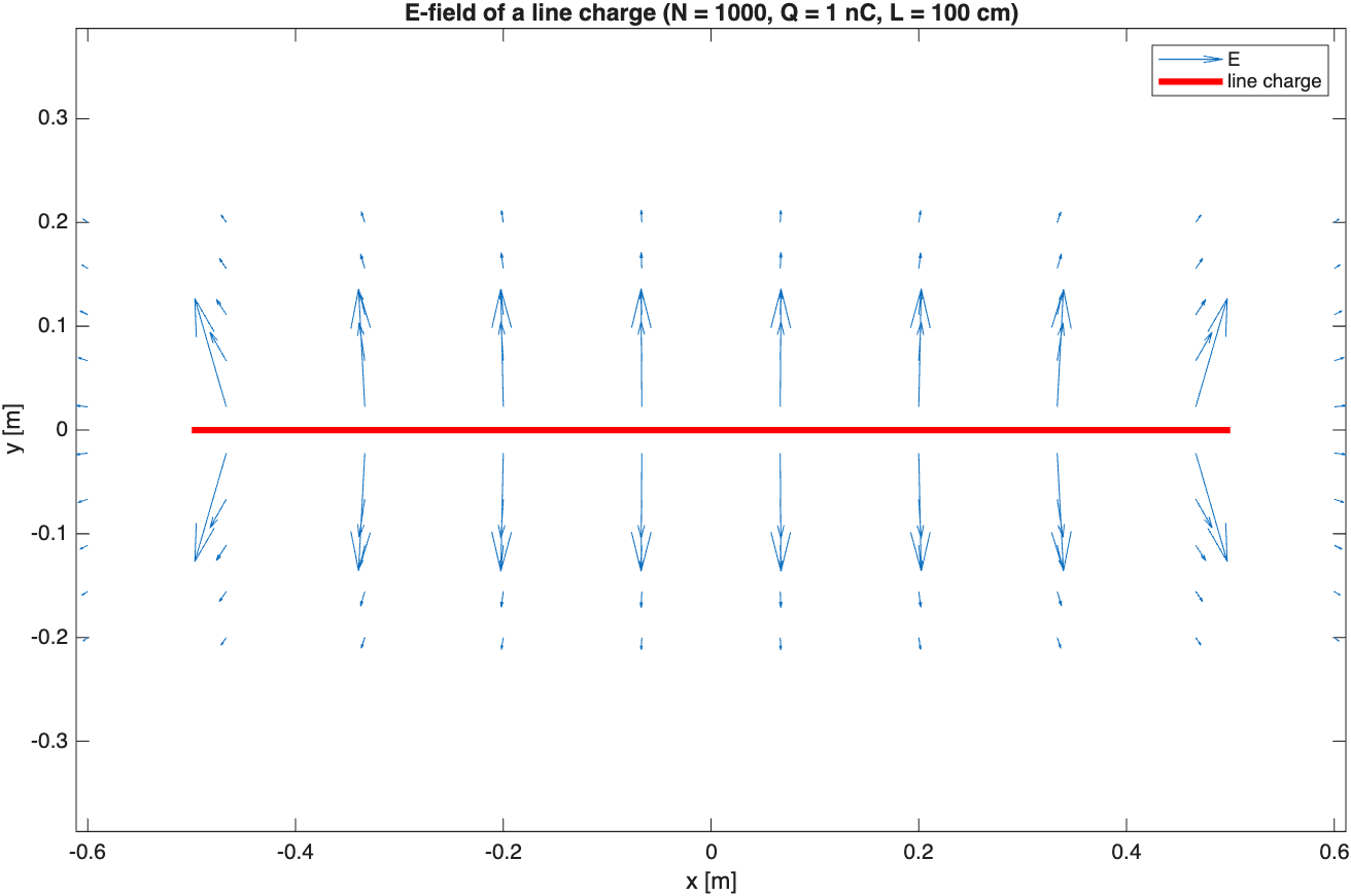
N = 1000, Q = 1 nC, L = 100 cm:
Q4 – Exercise 1.16: Finite vs infinite line charge
% MATLAB Exercise 1.16 - Finite vs infinite line charge.

% Finite line along z, centred at the origin; field points on the +x axis,

% so theta2 = -theta1 and only the x-component of (1.24) survives.

clear; clc;

eps0 = 8.8541878128e-12;


L = input('Length of the line L [cm]: ')/100;

rhol = input('Line charge density [nC/m]: ')*1e-9;


D = linspace(0.1*L, 2*L, 5000);

sinT2 = (L/2)./sqrt(D.^2 + (L/2)^2);

Efin = rhol./(4*pi*eps0*D) .* 2.*sinT2; % Eq. (1.24)

Einf = rhol./(2*pi*eps0*D); % Eq. (1.25)

err = (Einf - Efin)./Efin*100;


kmax = D(find(err > 10, 1))/L;

fprintf('\nL = %g m, rho_l = %g C/m\n', L, rhol);

fprintf('Error at k = 0.1: %.3f %%, at k = 2: %.3f %%\n', err(1), err(end));

fprintf('kmax (error > 10%%) = %.4f, Dmax = %.4f m\n', kmax, kmax*L);


figure;

plot(D/L, Efin, '-', D/L, Einf, '--');

xline(kmax, '-', sprintf('k = kmax = %.3f', kmax));

xlabel('k = D/L'); ylabel('E [V/m]');

title('Comparison of E-fields due to finite and infinite lines of charge');

legend('Finite', 'Infinite');
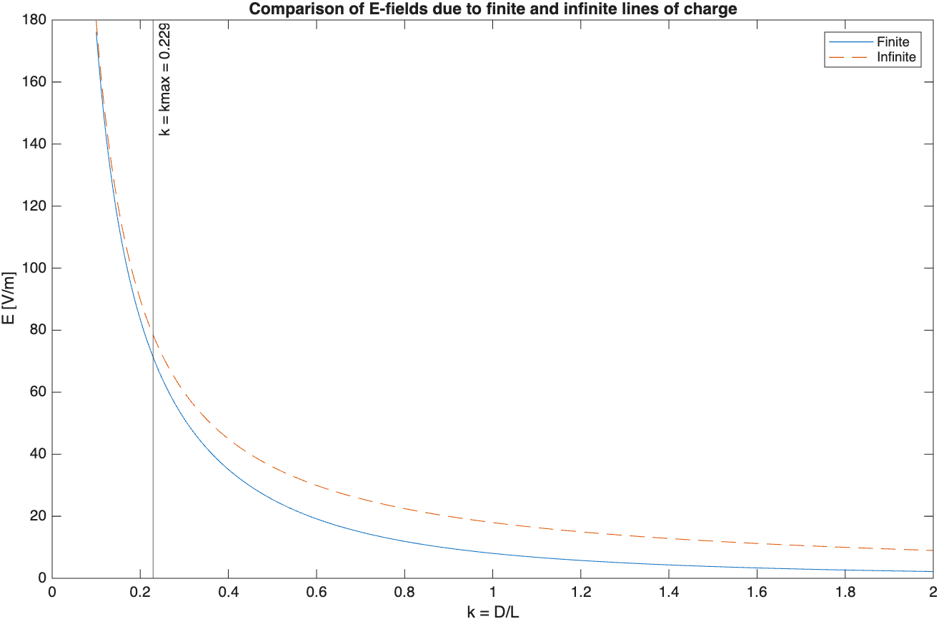
L = 100 cm, ρl = 1 nC/m. The error passes 10% at kmax = 0.229 (theory: √0.21 / 2 = 0.2291).
Q5 – Exercise 1.24: Coordinate conversion functions
| Function | Domain | Range |
|---|---|---|
| car2Cyl(x,y,z) | x, y, z ∈ ℝ | r ≥ 0, φ ∈ [0, 2π), z ∈ ℝ |
| car2Sph(x,y,z) | x, y, z ∈ ℝ | R ≥ 0, θ ∈ [0, π], φ ∈ [0, 2π) |
| cyl2Car(r,φ,z) | r ≥ 0, φ ∈ ℝ (rad), z ∈ ℝ | x, y, z ∈ ℝ |
| sph2Car(R,θ,φ) | R ≥ 0, θ, φ ∈ ℝ (rad) | x, y, z ∈ ℝ |
Special cases: at the origin θ = φ = 0. On the z-axis φ = 0, and on the −z axis θ = π. All functions work element-wise on arrays.
Q6 – Exercise 2.1: Permittivity pop-up menu
Q7 – Exercise 1.25: Coordinate conversion GUI
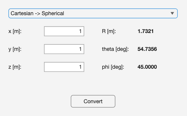
Cartesian (1, 1, 1) → spherical: R = √3, θ = 54.74°, φ = 45°.