Assignment 4

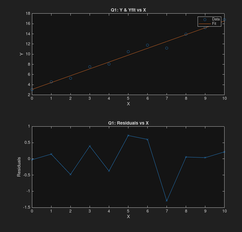
1. Table 1: Linear Fit ($Y={\beta }_0+{\beta }_{1}X$ )

Fit Results

• $bet{a}_0=3.0662$
• $bet{a}_1=1.3495$
• ($R^2$ = 0.984), Adjusted ($R^2$ = 0.983)
• RMSE = 0.593
• F-statistic = 569, p-value = ($1.90\times 10^{-9}$)

Fitted equation:

$$\hat{Y}=3.0662+1.3495X$$

ANOVA Table:

Source	SS	df	MS	F	p-value
Regression	MATLAB	1	–	569	$1.90\times 10^{-9}$
Residual	–	9	–
Total	–	10

---

Parameter SE and t-tests:

Param	Estimate	SE	t	p-value
β₀	3.0662	0.33457	9.1645	$7.36\times 10^{-6}$
β₁	1.3495	0.056553	23.863	$1.90\times 10^{-9}$

---

Matrix results:

$$(X^{\prime }X{)}^{-1}=\left[\begin{array}{cc}0.3182& -0.0455\\ -0.0455& 0.0091\end{array}\right]$$

---

2. Table 2: Fits

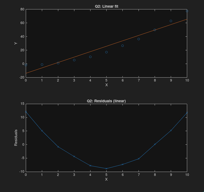
(a) Linear Fit ($Y={\beta }_0+{\beta }_{1}X$)

• $bet{a}_0=-13.956$
• $bet{a}_1=7.9646$
• ($R^2$ = 0.923), Adjusted ($R^2$ = 0.915)
• RMSE = 8.03
• F-statistic = 108, p-value = ($2.57\times 10^{-6}$)

Fitted equation:

$$\hat{Y}=-13.956+7.9646X$$

Parameter SE and t-tests:

Param	Estimate	SE	t	p-value
β₀	-13.956	4.5277	-3.0824	0.013089
β₁	7.9646	0.76533	10.407	($2.57\times 10^{-6}$)

---

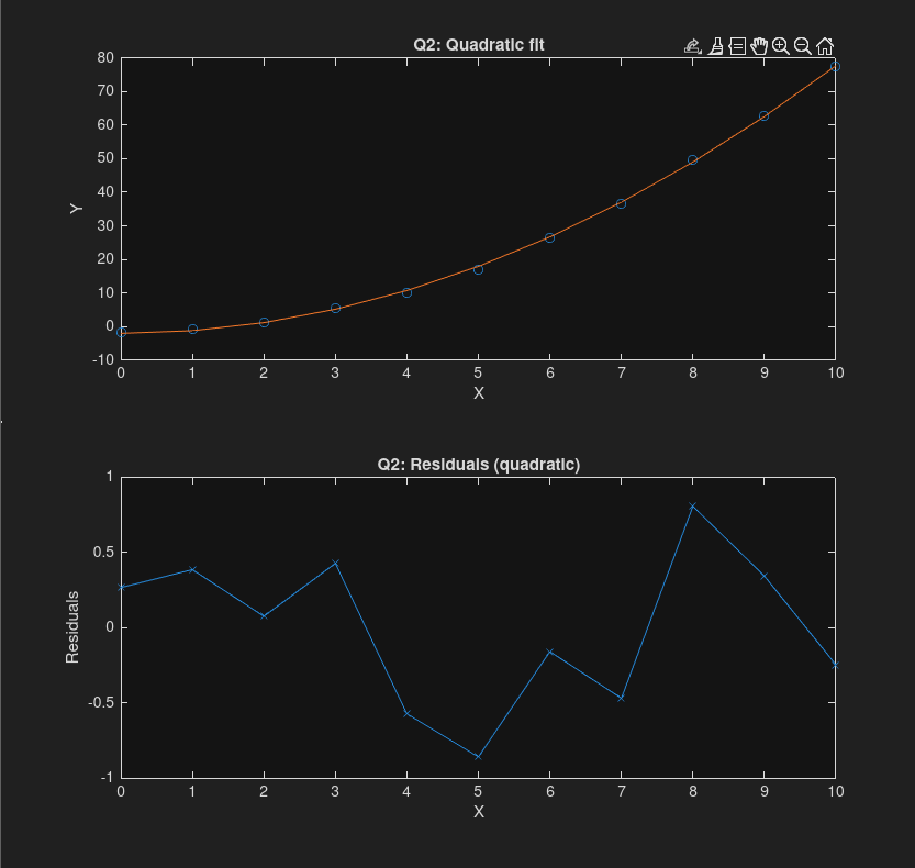
(b) Quadratic Fit ($Y={\beta }_0+{\beta }_1{X}^2$)

• Transform (Z = $X^2$)
• $bet{a}_0=-2.0705$
• $bet{a}_1=0.7982$
• $R^2\approx 1.000$, Adjusted ($R^2$ = 1.000)
• RMSE = 0.533
• F-statistic = ($2.66\times 10^4$), p-value = ($6.19\times 10^{-17}$)

Fitted equation:

$$\hat{Y}=-2.0705+0.7982X^2$$

Parameter SE and t-tests:

Param	Estimate	SE	t	p-value
β₀	-2.0705	0.23471	-8.8218	($1.01\times 10^{-5}$)
β₁	0.7982	0.0048908	163.21	($6.19\times 10^{-17}$)

---

(c) Model Comparison

• Linear model: High ($R^2$) but residuals show curvature → poor fit at large
• Quadratic model: ($R^2\approx 1$), residuals random, very small RMSE.
• Conclusion: Quadratic model is the better fit. Residual analysis confirms.